Is fractal interpolation effective to recover missing data?
Introduction
Unfortunately, it is a common occurrence that the data a data analyst has is incomplete.
This missing data has to be filled out a certain way and then the work is done with the “new” data. However, it may happen that the resulting data significantly distorts the real one. Thus, it will obviously lead to a loss in quality for the models based on this data. Therefore, finding the optimal solution to the missing values problem is a very important task. In this article, we will talk about different ways of filling in the missing data and how to compare the results obtained by different methods and on various open datasets.
A few words about interpolation
According to Wikipedia, interpolation is a method of constructing new data points within the range of a discrete set of known data points.
We will take a look at one-dimensional interpolation, which will be in finding the function of one real variable passing through a given set of points in the plane.
Next, we briefly touch upon the basic interpolation methods. Let’s note that the interp1d class is implemented in the scipy.interpolate package to perform one-dimensional interpolation using various methods.
Nearest-neighbor interpolation is the simplest interpolation method. Its essence is that it selects the nearest known function value as an intermediate value:
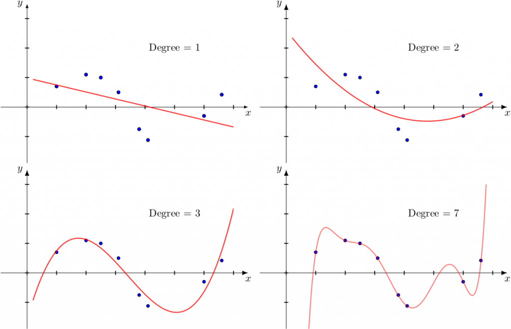
Polynomial interpolation is another interpolation method. It is well known from the higher mathematics course that if there is a set of N points of the plane (with pairwise distinct abscissas), then there is a single polynomial of degree N-1 passing through the indicated points. For example, if there are two points, then there is a unique line (a first-degree polynomial) passing through these points. There are formulas for finding such polynomials (for instance, Lagrange polynomial).
In reality, a situation referred to as “overfitting” will occur for large enough N points. The following illustration demonstrates this (data marked with blue dots and generated from y=sin(x), the red curve is an polynomial interpolation with degree 1, 2, 3 and 7; we see that the best interpolation for polynomial degree 3 and observe overfitting for the polynomial degree 7):
Spline interpolation can be used in order to avoid overfitting. In this interpolation method, at each interval between the interpolation points, the interpolation function is a polynomial, which the degree is limited (for example, in cubic interpolation, this is a polynomial of degree less than 3). Since this kind of interpolation is ambiguous, additional conditions are imposed on the resulting function, for example, differentiability at interpolation points.
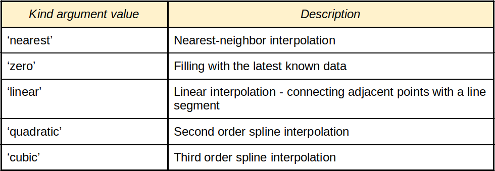
Interpolation methods, determined by the value of the argument “kind” for the class scipy.interpolate.interp1
Fractal interpolation
Fractal interpolation is another method that was proposed by the American mathematician Michael Barnsley in the mid-1980s. This method is described in a series of his articles and the wonderful book “Fractals Everywhere”. There the interpolation occurs by the so-called fractal self-affine functions. Let us briefly describe the nature of such mathematical objects.
About self-similar, self-affine sets, and fractals
What is a self-similar set? It’s a set which consists of several parts, each of which is a reduced copy of the set itself. Mathematically speaking, each of these parts is an image of the original set with a certain similarity transformation.
Cantor set is the most famous self-similar set (probably because historically it was the very first). It has the following construction. From a unit interval let’s remove the middle third, which is the interval
. The remaining set is the union of the two intervals. Now, we remove the middle third from each segment. Thus, obtaining a new set, which is the union of four intervals. Then repeat this procedure. By removing the middle thirds of all four intervals, we get a new set. Those points that are never left out of a single segment form a Cantor set.

It is easy to understand that the part of the Cantor set that belongs to the segment (like the one that belongs
) is similar to the original set (i.e. it is obtained from the original set by compression with the coefficient
).
The specified property is a characteristic of the Cantor set. More strictly – two contraction mappings of
. Then there’s the unique set
such that
. This set is a Cantor set.
However, we are more interested in sets on the plane. Sierpinski carpet is the simplest example of a self-similar set on a plane where a similar procedure, as in the case of a Cantor set, occurs with a unit square:
The Sierpinski carpet is a self-similar set, for it can be represented as a union of eight reduced copies of itself.
A rather general idea of specifying self-similar sets was probably first described in the article J. Hutchinson “Fractals and self similarity” in 1981. Some time later, Hutchinson’s ideas were developed by M. Barnsley. To some extent, he replaced similarity transformations with affine transformations. As a result, self-affine sets became the natural generalization of self-similar sets. Now such sets are called fractals. An outstanding mathematician Benoit Mandelbrot introduced this term into scientific use in the 70s of the twentieth century. By the fractal, Mandelbrot meant objects that have to some extent self-similar properties. Often, fractal sets are graphs of some continuous functions. Such functions, which graphs are fractal sets, are usually called fractal functions.
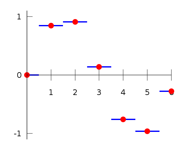
Let’s take a look at one of the simplest examples of a fractal function. Construct a sequence of functions on the segment . Suppose
is the diagonal of a unit square (see figure below). Function
is obtained from
by replacing a graph segment with a broken line of three links connecting the points
. With each of the resulting graph of the function
repeat the same procedure and get the function graph
, etc.
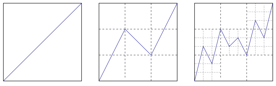
From the course of mathematical analysis, it is known that the resulting functional sequence has a limit, and it is also a continuous function. Furthermore, this is one of the simplest examples of a continuous nowhere differentiable function, first described in the monograph N. Bourbaki “Functions of a Real Variable”. Now it’s also known as Katsuura function.
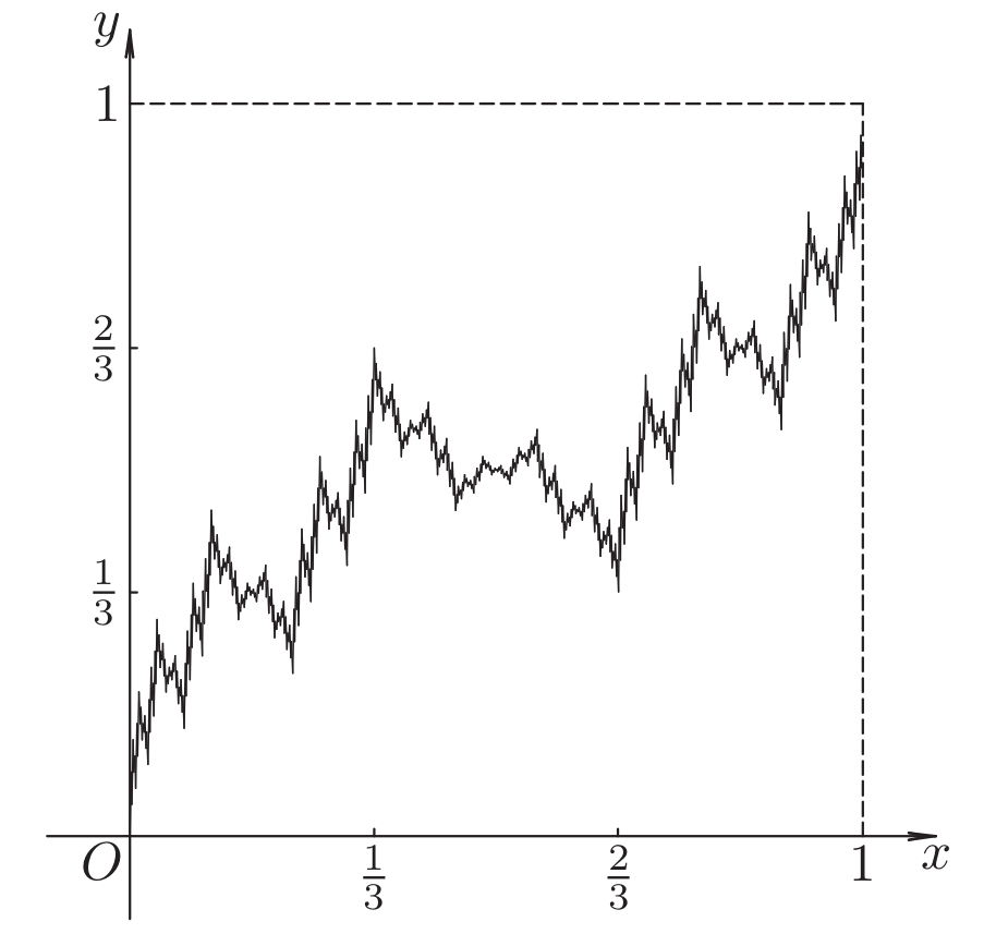
The described function is a particular example of self-affine functions. In fact, if we designate as a graph of the limit function, then
,
where
As in the case of self-similar sets, in order to define a self-affine function, it suffices to specify a certain set of contracting affine transformations of the plane. M. Barnsley used this idea, defining fractal interpolation functions. More details on how to define such functions can be found in the article Curve Fitting by Fractal Interpolation (P. Manousopoulos, V. Drakopoulos, T. Theoharis).
The interpolation method is as follows: the data set matches the set of plane transformations
of the type
Here
are free parameters, and the remaining coefficients are uniquely determined by the
from the conditions
and
.
It is known, that if are contraction mappings, then the operator W is contractive and has a unique fixed point in the space of compact sets of with the Hausdorff metric. Barnsley showed that if
, then mappings are contractive in some metric on
. In this case, the fixed point of the constructed operator, i.e. compact set
satisfying the condition
, will be a graph of continuous function f, which interpolates the initial data.
So, if we have a set of points on the plane, then there is a whole class of fractal interpolation functions interpolating them. Various sets of free parameters will spawn various functions.
Finding methodology of the optimal fractal interpolation function
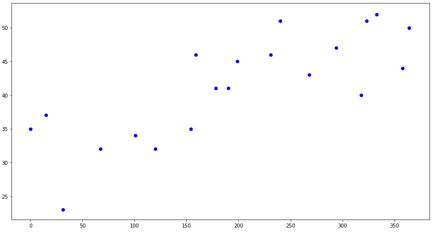
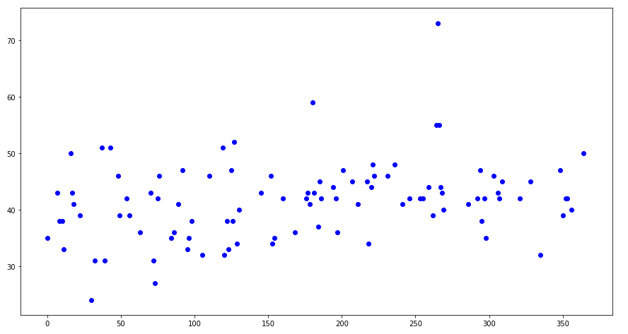
Example 1. Initial data: Daily total female births in California in 1959. The initial data set contains 365 points:
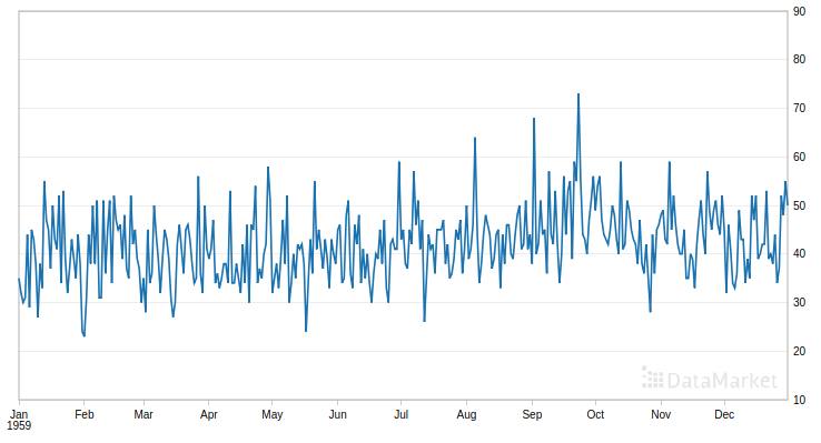
We include randomly selected 20 points in the known data:
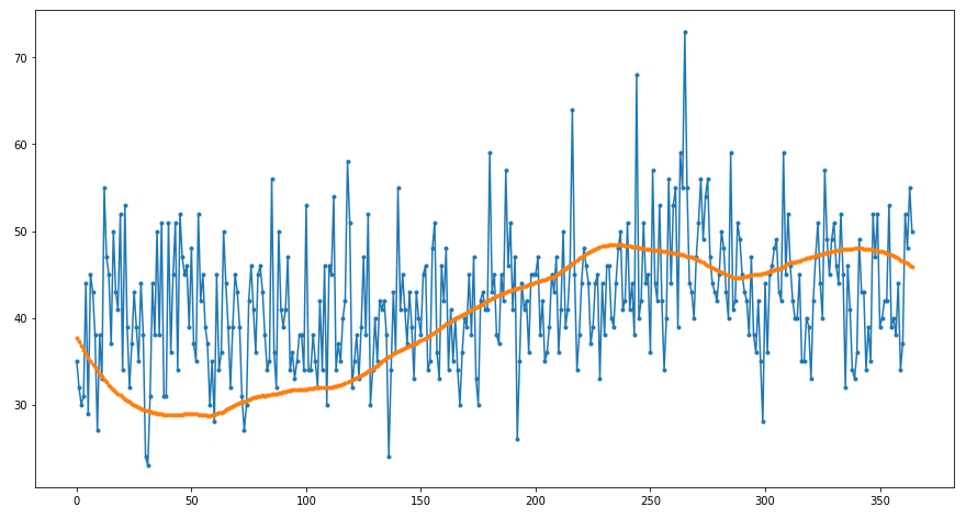
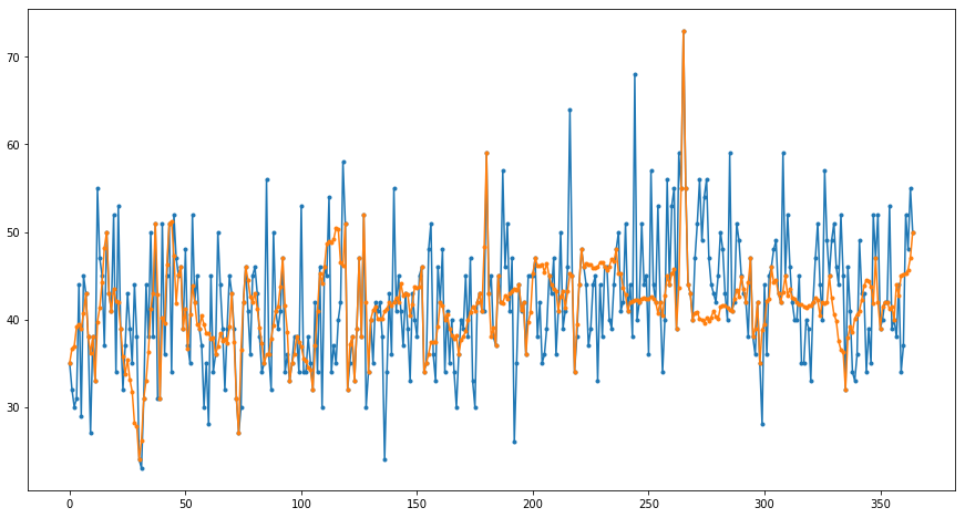
The result of the fractal interpolation is presented in the figure:
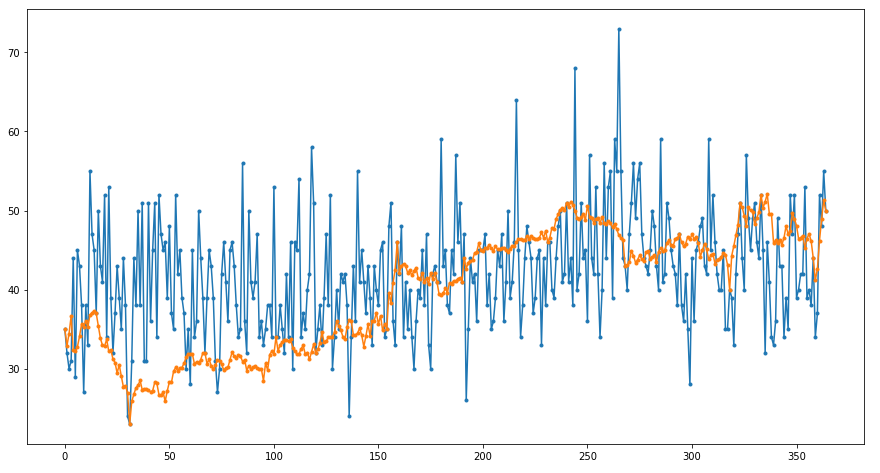
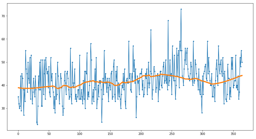
After applying the Savitzky-Golay filter, we obtain such a smooth curve:
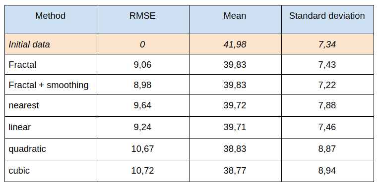
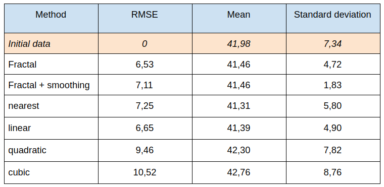
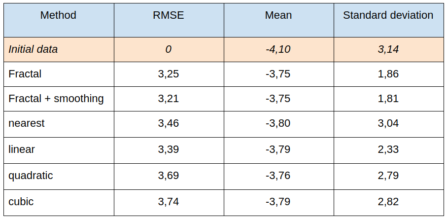
Next table presents the root-mean-square error, mean and standard deviation, calculated for different interpolation methods:
Example 2. The same data set, values at 100 points are known:
The result of fractal interpolation:
and after smooting:
As you can see, the result of smoothing does not meet expectations. However, let’s take a look at the statistical indicators and the error of various interpolation methods:
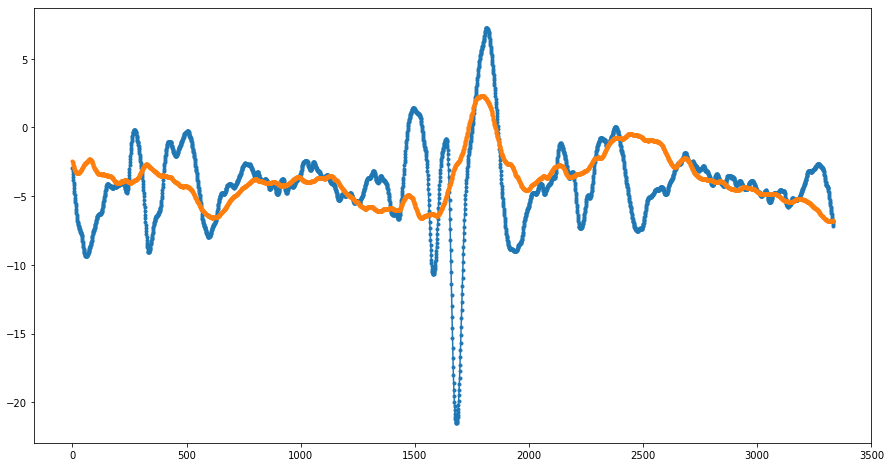
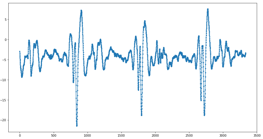
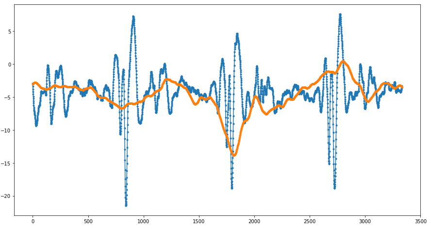
Example 3. Initial data is a fragment of electrocardiogram data of one of the patients (data is taken from CEBS database).
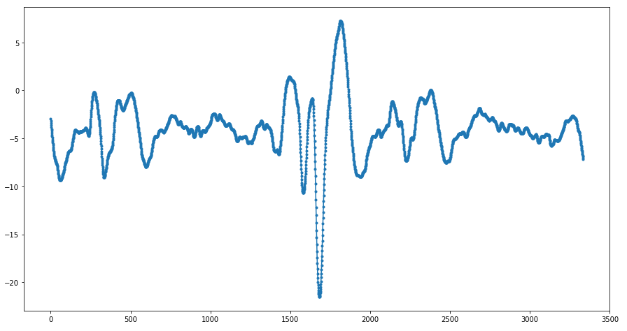
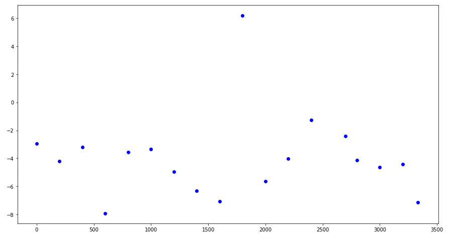
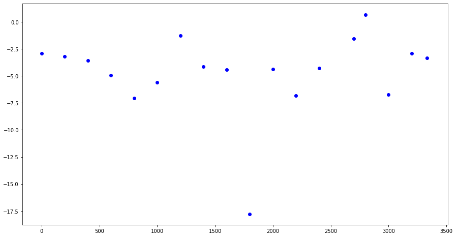
The data consists of 3333 points. We leave only the uniformly distributed 18 points and interpolate the data at these points:
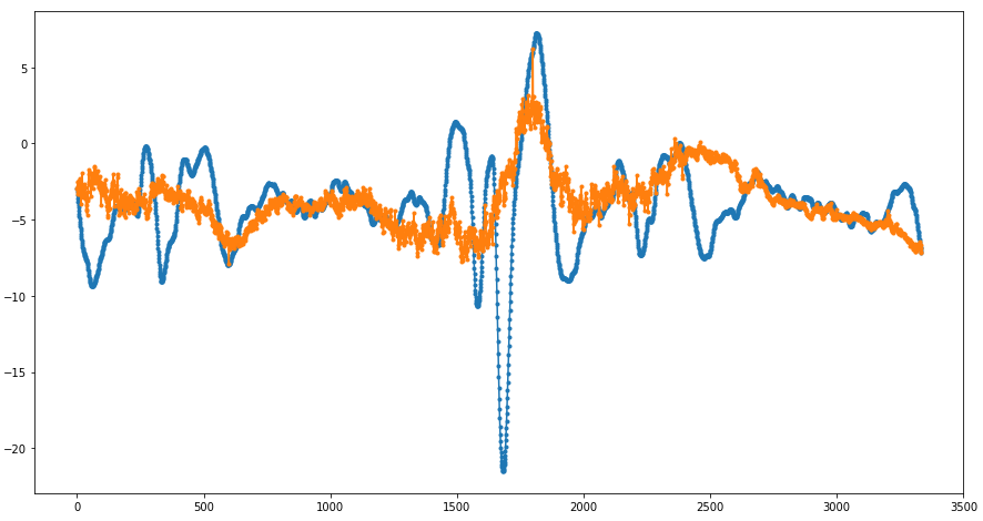
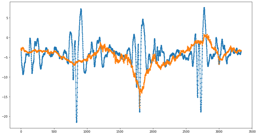
The results of fractal interpolation (before and after smoothing) are presented in the following figures:
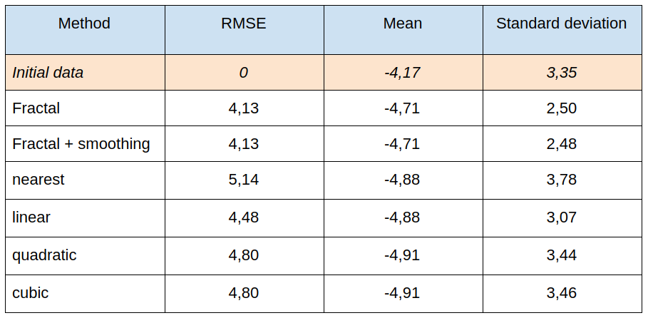
For comparison, let’s take a look at the standard interpolation methods:
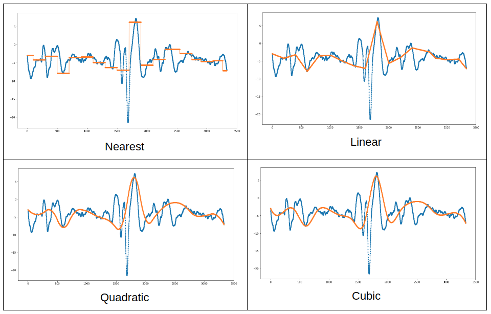
Let’s compare the results of this interpolation with the traditional ones:
Example 4. Initial data: a fragment of electrocardiogram data from one of the patients (data is taken from CEBS database). The initial data consisted of 20,000 consecutive values, but we left only every sixth point:
As before, we leave only the evenly distributed 18 points and interpolate the data at these points:
The results of fractal interpolation (before and after smoothing) are presented in the following figures:
Again, we compare the results of this interpolation with the traditional ones:
Conclusion
The examples show slightly better total error values with fractal interpolation than with conventional methods. At the same time, a “miracle” didn’t happen, for the error value, although better, it’s not “way better”.
We also tried to interpolate points of a randomly chosen fractal interpolation function (with random free parameter initialization). The result is worse and is comparable with traditional interpolation methods. The result worsens and becomes comparable with the traditional.
If the data values at each next step in general do not depend on the value at the previous point (as in examples 1 and 2), then it is better to leave out the smoothing. Such a process is just more logical to think of a non-differentiable, and therefore fractal function. If the nature of the data is such that it is convenient to describe them with a continuous and differentiable function, then after the fractal interpolation it is better to perform smoothing.
-
Time consuming. The search for the optimal interpolation function is resource-intensive because at each step a search is made for a set of free parameters in which the function best suits the artificially missing value.
-
The fractal interpolation function that best describes the value at the artificially missing point may result in “overfitting”.
The described cons attract our attention to building the best algorithms to find fractal interpolation functions. It is possible that this will require new restrictions on them. Particularly, such restriction could be the fractal dimension of the resulting graph, i.e. the search for the fractal interpolation function is performed in the class of functions with a predetermined fractal dimension (for example, box-counting dimension). Preventing the fractal dimension of the graph from exceeding the predetermined number can serve as an element of regularization and prevent overfitting.
Hy!
I’m very interested in the topic and want to use some of the ideas mentioned here in my PhD research.
Can you maybe send me the programs you used for doing these interpolations?
And do you maybe have some more corresponding references?
All the best Sebastian